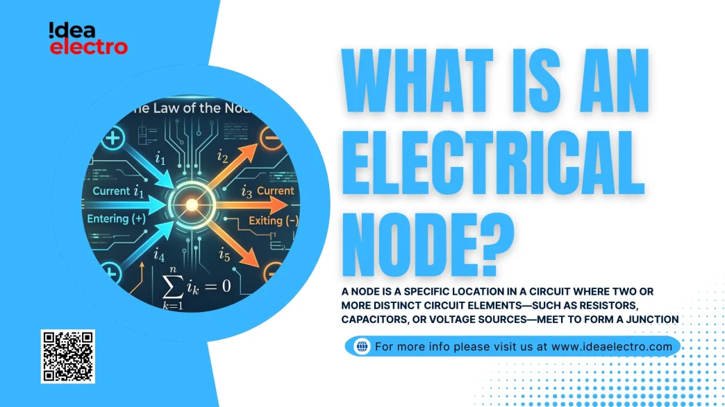
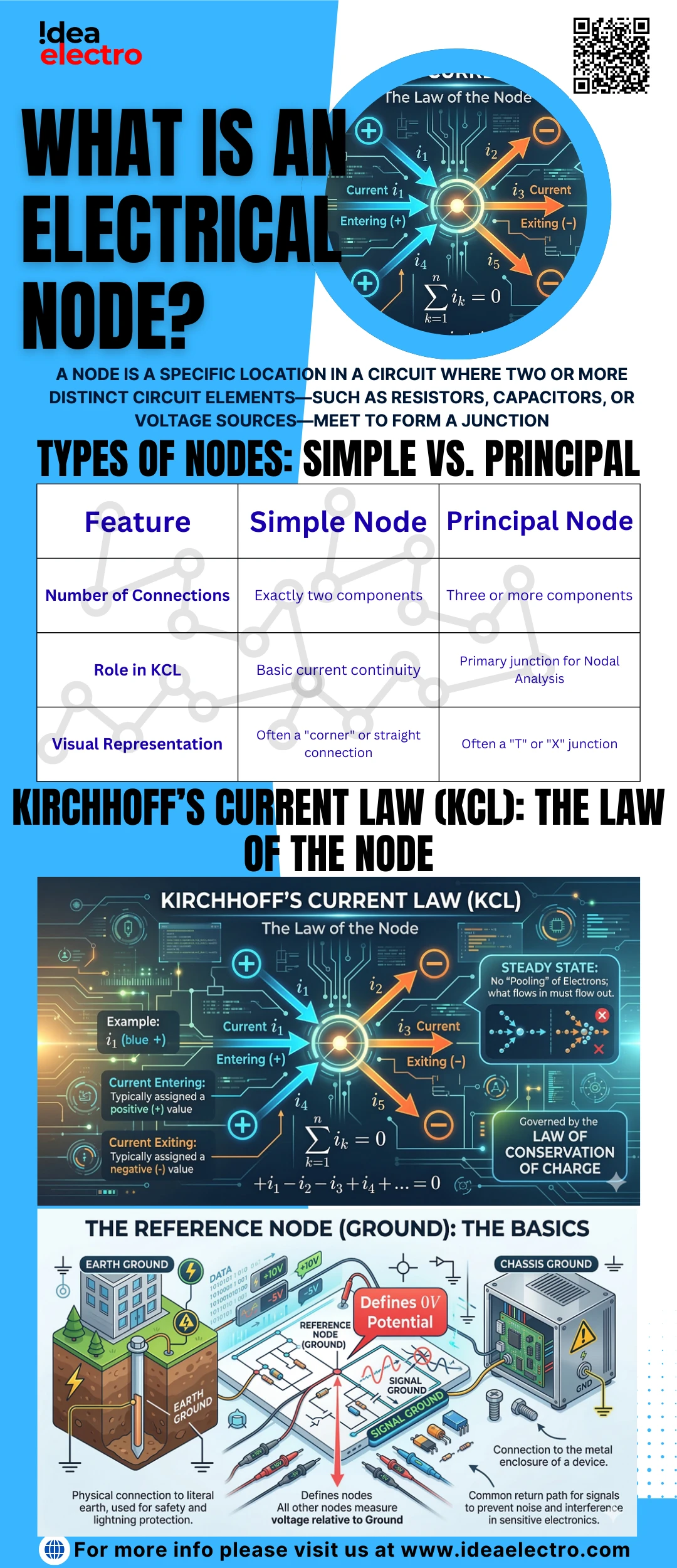
The study of electrical networks begins with understanding the fundamental point of connection known as a node. In its simplest terms, a node is a specific location in a circuit where two or more distinct circuit elements—such as resistors, capacitors, or voltage sources—meet to form a junction. While beginners often visualize a node as a single dot on a schematic, circuit theory treats a node as an equipotential surface. This means that regardless of the physical length of the connecting wire, every point on that wire maintains the same electrical potential (voltage) relative to a reference. This concept is foundational to Nodal Analysis, a method used widely in engineering to determine the voltages throughout a system. Understanding nodes allows engineers to simplify complex physical layouts into manageable mathematical models.
Moving beyond the visual “dot” on a paper, the technical definition of a node encompasses all interconnected conductive paths that have no components between them. In an ideal circuit model, we utilize the “Ideal Wire” assumption, which posits that wires have zero resistance ($R = 0$). Because there is no resistance, there is no voltage drop across the wire itself ($V = I \times R$), meaning the entire conductive segment is one single node. If you can trace your finger along a wire without crossing a component like a resistor or a battery, you are still on the same node. This distinction is vital because a single node can span across a large physical area of a circuit board, yet it remains a single electrical entity in calculations.
Definition: Electrical Node
A node is the entire junction or connection point where two or more circuit components are joined together. In circuit schematics, any group of wires connected directly together (with no intervening components) constitutes a single node, characterized by having a uniform electrical potential across its entire boundary.
Types of Nodes: Simple vs. Principal
In circuit analysis, not all nodes are treated with the same level of priority. Engineers categorize them based on the number of branches they connect to streamline the solving process.
| Feature | Simple Node | Principal Node |
| Number of Connections | Exactly two components | Three or more components |
| Role in KCL | Basic current continuity | Primary junction for Nodal Analysis |
| Visual Representation | Often a “corner” or straight connection | Often a “T” or “X” junction |
- Simple Node: These occur where only two elements meet, such as two resistors in series. While they are technically nodes, they are often bypassed in complex matrix calculations because the current entering must equal the current leaving through the only other available path.
- Principal Node: These are the critical junctions where three or more branches converge. These are the focal points for Kirchhoff’s laws because they represent the points where current actually “splits” or “combines”. Identifying principal nodes is the first step in reducing the number of simultaneous equations needed to solve a circuit.
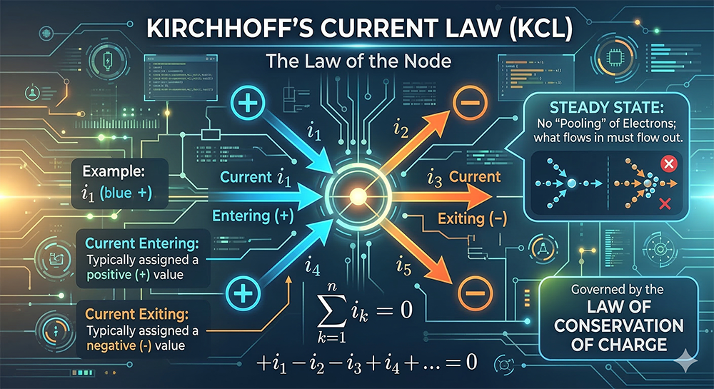
Kirchhoff’s Current Law (KCL): The Law of the Node
Kirchhoff’s Current Law (KCL) serves as the primary governing principle for nodes. It states that because a node has no mass or volume to store electrical charge, the total charge entering a node must instantaneously equal the total charge leaving it. This is a direct application of the Law of Conservation of Charge. Mathematically, the algebraic sum of all currents entering and exiting a node is zero:
$$\sum_{k=1}^{n} i_k = 0$$
To apply this law correctly, engineers use a specific sign convention to maintain consistency during calculation:
- Current Entering: Typically assigned a positive ($+$) value.
- Current Exiting: Typically assigned a negative ($-$) value.
- Steady State: KCL assumes that no “pooling” of electrons occurs; what flows in must flow out.
Identifying Nodes in Complex Schematics
Identifying nodes in a complex drawing can be daunting for students who see “loops” instead of “junctions.” Follow these systematic steps to clarify the schematic:
- Locate all Components: Start by identifying every resistor, capacitor, inductor, and power source. These are the “boundaries” that separate one node from another.
- Trace Continuous Copper: Use a colored highlighter to trace along a wire. Continue tracing until you hit a component. Everything you have colored in one continuous stroke is one single node.
- Labeling: Assign a letter or number to each unique colored area (e.g., Node A, Node B). If two points are connected by a wire with no component between them, they are the same node, even if they look far apart on the diagram.
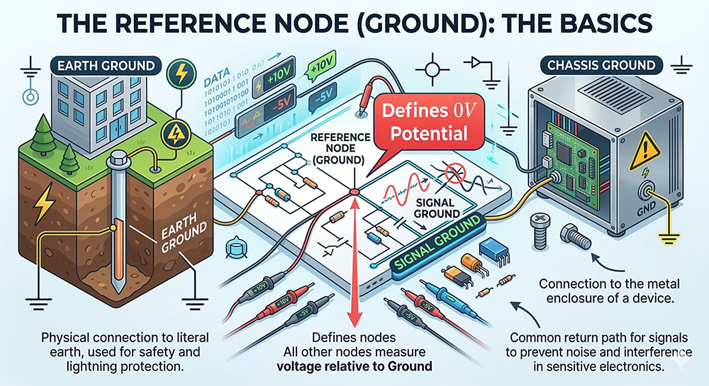
The Reference Node (Ground)
In every practical circuit analysis, one node must be chosen as a reference point, commonly referred to as Ground. We define the potential at this node as $0V$, allowing us to measure the voltage of all other nodes relative to this baseline.
- Earth Ground: A physical connection to the literal earth, used for safety and lightning protection.
- Chassis Ground: A connection to the metal enclosure of a device.
- Signal Ground: A common return path for signals to prevent noise and interference in sensitive electronics.
Common Pitfalls for Beginners
Even with a clear definition, certain mistakes frequently occur during the learning process:
- The “Long Wire” Mistake: Beginners often treat a long wire on a schematic as multiple nodes.
- Correction: If there is no component between two points on a wire, they are the same node, no matter how long the line is drawn.
- Ignoring Series Nodes: Some students ignore the node between two resistors in series because they think it “doesn’t do anything.”
- Correction: Even if the current is the same, the voltage changes across each component; identifying this node is essential for finding the voltage drop.
Conclusion
Mastering the concept of the electrical node is the definitive “first step” toward proficiency in electrical engineering. By recognizing nodes as equipotential surfaces rather than just physical dots, you unlock the ability to perform Nodal Analysis and accurately simulate complex systems. This foundational understanding ensures that as circuits grow in complexity, your mathematical model remains grounded in the physical laws of conservation.